Principal Component Analysis: Derived and Coded
Principal Component Analysis (PCA) is a method to get low dimensional representation of a high-dimensional dataset without losing the important features. PCA can be useful for visualization of the dataset or determining features from data. More formally, if we are given data set of $n$ original $d$-dimensional points $X = \{x_1,\dots,x_n\} \in \mathbb{R}^{n\times d}$, we want to obtain $n$ new $k$-dimensional points $Z = \{z_1, \dots, z_n\} \in \mathbb{R}^{n\times k}$ with $k\ll d$, for which the projection back onto the original dimension $d$: $\bar X = \{\bar x_1,\dots,\bar x_n\} \in \mathbb{R}^{n\times d}$, is as close as possible to the original data $X$.
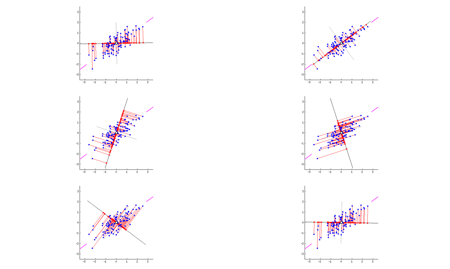
between $\bar X$ and $X$ [builtin.com]
Theoretical derivation
For the next derivation, let’s assume the data is standardized (i.e., mean $\mu = 0$ and standard deviation $\sigma = 1$). Our goal is to minimize the squared Euclidean distance $\left\lVert wz_i - x_i\right\rVert_2^2$ between each projected point $\bar x_i = wz_i$ and original point $x_i$, where $w$ is a unit vector ($\left\lVert w \right\rVert_2 = 1$) and $z_i$ are the lower-dimensional coordinates:
\[\left(\boldsymbol{w}^*, \mathbf{z}^*\right)=\arg \min _{\left\lVert \boldsymbol{w} \right\rVert_2=1, \mathbf{z}} \sum_{i=1}^n\left\| \boldsymbol{w}z_i-\boldsymbol{x}_i\right\|_2^2\]We assumed $\left\lVert w \right\rVert_2 = 1$, because for any fixed $\left\lVert w \right\rVert_2 = 1$ it holds that $z_i^* = \textbf{w}^Tx_i$. Our term is now therefore only minimizing over the $w$’s. We get
\[\begin{align} w^* &=\arg \min _{\left\lVert \boldsymbol{w} \right\rVert_2=1} \sum_{i=1}^n\left\| \boldsymbol{w}w^Tx_i-\boldsymbol{x}_i\right\|_2^2 \\ &= \arg \min_{\left\lVert w \right\rVert_2 = 1}\sum_{i=1}^n \left\lVert x_i \right\rVert_2 - \sum_{i=1}^n(w^\top x_i)^2 \\ &= \arg \max _{\left\lVert \boldsymbol{w} \right\rVert_2=1} \sum _{i=1}^n (w^Tx_i)^2 \\ &= \arg \max _{\|\boldsymbol{w}\|_2=1} w^T \Big( \underbrace{\sum _{i=1}^n x_i x_i^T}_{n\Sigma} \Big)w \\ \end{align}\]where $\Sigma = \frac{1}{n}\sum_{i=1}^{n}x_ix_i^T$ is the covariance for $\mu = 0$ (data is centered). And now the optimal solution to $w^* =\arg \max _{\left\lVert \boldsymbol{w} \right\rVert_2=1} w^T \Sigma w$ is given by the principal eigenvector of $n\Sigma$. This means we can perform SVD decomposition of the Covariance matrix and extract the principal eigenvector (eigenvector corresponding to the highest eigenvalue).
SVD decomposition of matrix $A$ is a representation of that matrix as \(A = USV^\top\) where $U,V$ are orthogonal matrices and $S$ is diagonal matrix with singular values. We can (together with eigenvectors) reorder them such that $\lambda_1 \geq \lambda_2 \geq \dots \lambda_d \geq 0$. That will be important for the next step.
Hence the SVD decomposition goes as follows:
\[n \Sigma={X}^T {X}={V} {S}^T \underbrace{U^T U}_{=I\ (\text{orthogonal})} {S} {V}^T={V} {S}^T {S} {V}^T={V} {D} {V}^T\]And so (assuming the decreasing order of the eigenvalues) the solution is given by $v_1$ for $k=1$ - the first column of $V = (v_1, \dots, v_d)$ from the SVD, the eigenvector corresponding to the biggest eigenvalue. This is the vector carrying the most amount of information about the dataset. In case of PCA for $k\geq1$, the problem generalizes into
\[(W^*,Z) = \arg\min_{W^\top W = I, Z} \sum_{i=1}^n \left\lVert Wz_i - x_i \right\rVert_2^2\]We can solve it analogously to $k=1$.
-
Obtaining $W$ - We can generalize the previous case for $k=1$ and say that the solution is given by $k$ eigenvectors corresponging the $k$ largest eigenvalues of the SVD decomposition on $X^\top X$, i.e. $W = (w_1, \dots, w_k)$
-
Obtaining $Z$ - As we already know how to get $z_i$ using $w$ from the $k=1$ case, it generalizes into $z_i = W^\top x_i$ for all $i=1,\dots ,n$, i.e. $Z = W^\top \cdot X$
Shortly summarized, we need to
- Standardize the data
- Compute the Covariance matrix of $X$
- Decompose this matrix to get $k$ eigenvectors corresponding to the $k$ highest eigenvalues
- Stack them vertically to get matrix $W = (w_1, \dots, w_k)$
- Project the original data to obtain $ Z = (z_1,\dots,z_n)$
Manual PCA Implementation
Let’s implement PCA from scratch (with NumPy) to better understand how it works under the hood.
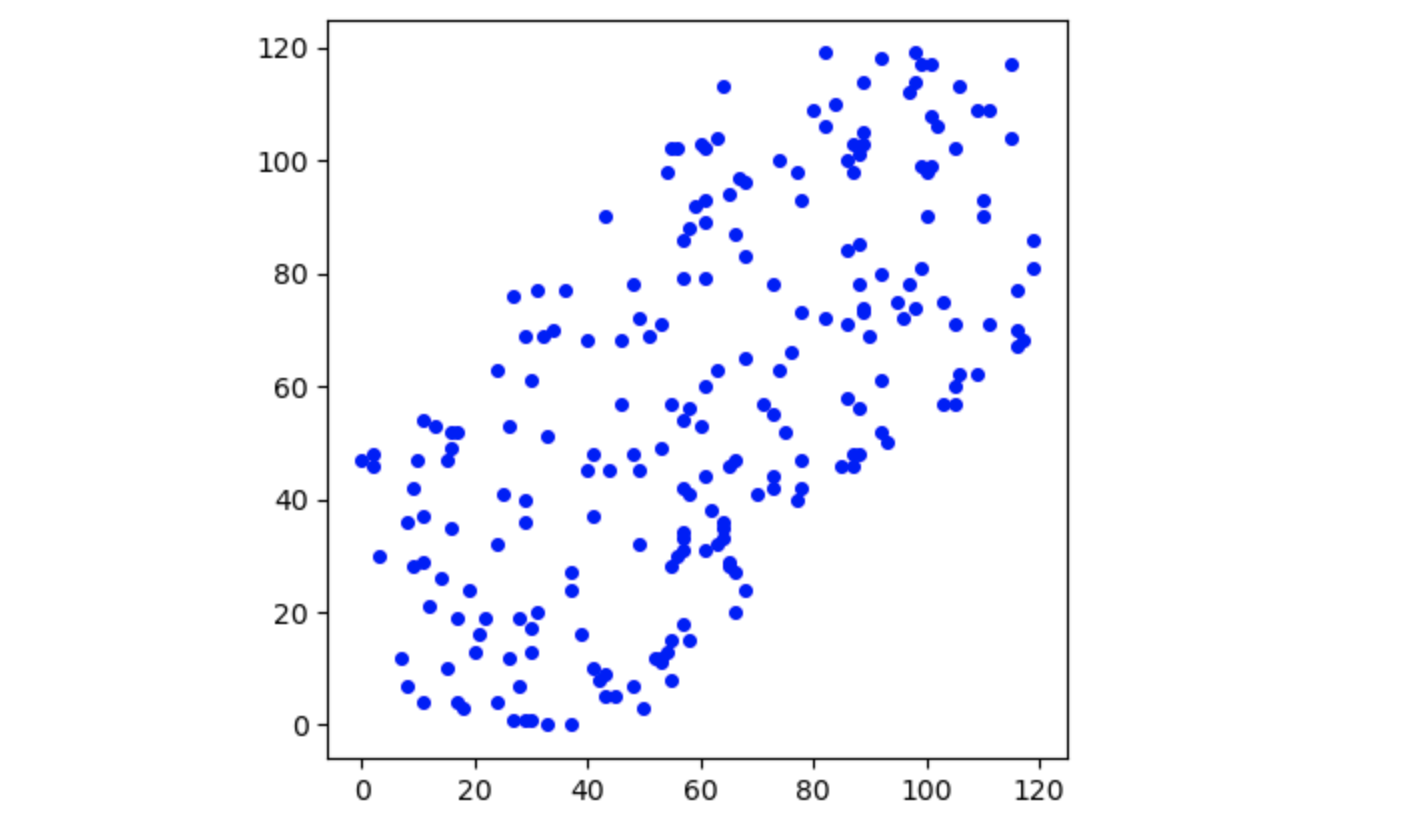
To make this implementation demonstration a little more robust, we will no longer assume standardized data. I will demonstrate each part of the implementation on an example. Let’s say we want to perform PCA with $k=1$ on the following dataset $X$. First, we need to standardize the data. This is nothing more than substracting the mean and dividing by the standard deviation of the dataset.
X = (X-np.mean(X, axis=0)) / np.std(X, axis=0)
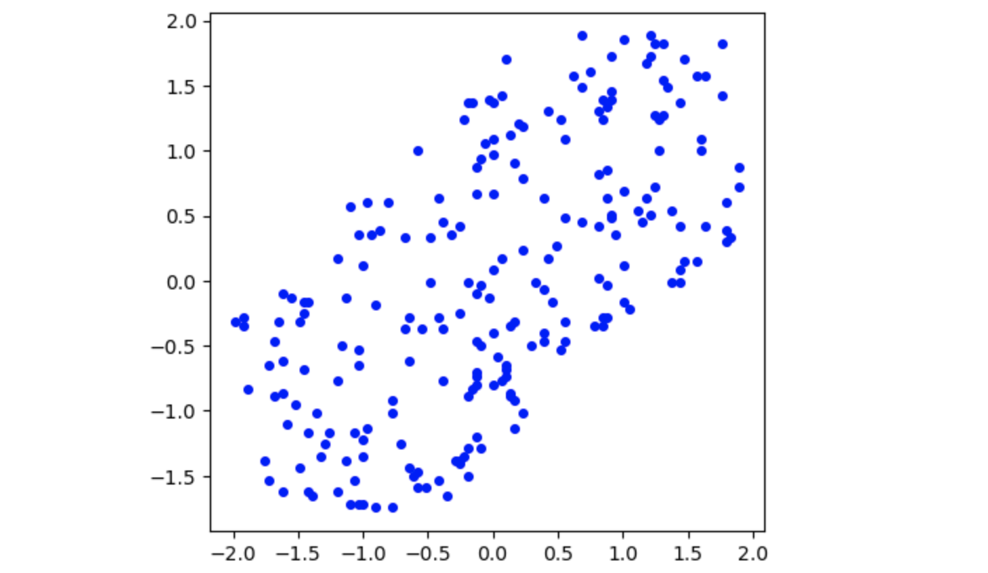
If we plot the data now, we notice that the plot looks exactly the same, only the axes shifted and the distance between points shrunk.
Covariance matrix. Computing the covariance matrix has now become easier since $\mathbb{E}[X]=0$ and $\text{Var}(X)=1$. All we need is:
\[Cov = \frac{X^\top X}{n} \quad n=\text{number of points}\]def cov_of_standardized(X):
n = X.shape[0]
return np.dot(X.T,X)/(n)
cov_X = cov_of_standardized(X)
For this particular dataset, the covariance matrix looks like this:
\[Cov_X = \begin{bmatrix} 1 & 0.62 \\ 0.62 & 1 \end{bmatrix}\]This is not a suprising result as the covariance matrix of X is a square matrix where the diagonal elements are the variances of the variables. Since each standardized variable has a variance of 1, the diagonal elements of the covariance matrix of a standardized dataset are all 1.
Eigenvectors of the Covariance Matrix. Just for fun, let’s see the eigenvalues (we expect two) and the corresponding eigenvectors (we expect 2x(1,2) vectors):
U,s,Vt = np.linalg.svd(cov_X)
print(U)
print(s)

>>> [179.23427235  41.76572765] # eigenvalues
>>> [[-0.70710678 -0.70710678]  # first eigenvector
>>>  [-0.70710678  0.70710678]] # second eigenvector
It might be a little abstract what we just did, so let’s look at the eigenvectors (these are the principal components) in the plane. They are scaled respectively to their eigenvalue. The blue vector is the [-0.70710678 0.70710678] component and the red one corresponds to the [-0.70710678 -0.70710678] component.
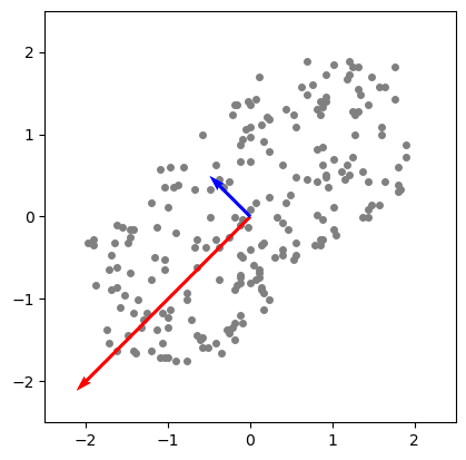
As already described above, we’re interested in extracting the k eigenvectors with the k largest corresponding eigenvalue.
Since the $k=1$ here, we expect the max of both value (and hence its eigenvector [-0.70710678, -0.70710678] to be extracted). Let’s translate to code.
u,s,vt = np.linalg.svd(mat)
indices = np.argsort(s) # returns indices from *smallest* to biggest EValue
indices = np.flip(indices,0)[:k] # (data, axis) and up to k-th index
W = np.real(u[:,indices])
return W
And indeed, what is returned is the expected eigenvector.
>>> [-0.70710678, -0.70710678]
Mapping the data. Now we can project the data onto the principal component.
Z = np.dot(X,W)
X_projected = np.dot(W, Z.T)
That’s it! We can plot the new points $(z_1, \dots, z_n)$ in orange against the original points in blue to visualize $Z$. We can do the same also with the re-projected points $(\bar x_1, \dots, \bar x_n)$ (distance of which from original dataset we wanted to minimize) and get a nice visualization of the dimension reduction.
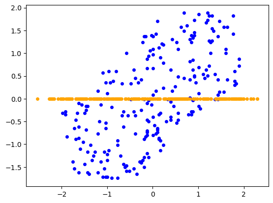
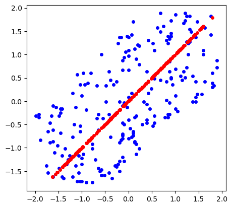
Important to notice - we are only considering the bigger eigenvalue for this dimension reduction. This means the larger eigenvalue is contains around 179.23 / (179.23 + 41.76) $\approx$ 81% of the information about the original dataset. This can be useful if we want for example to sustain given percentage of the original dataset features - we can choose $k$, such that the sum of the eigenvalues satisfies the percentage.